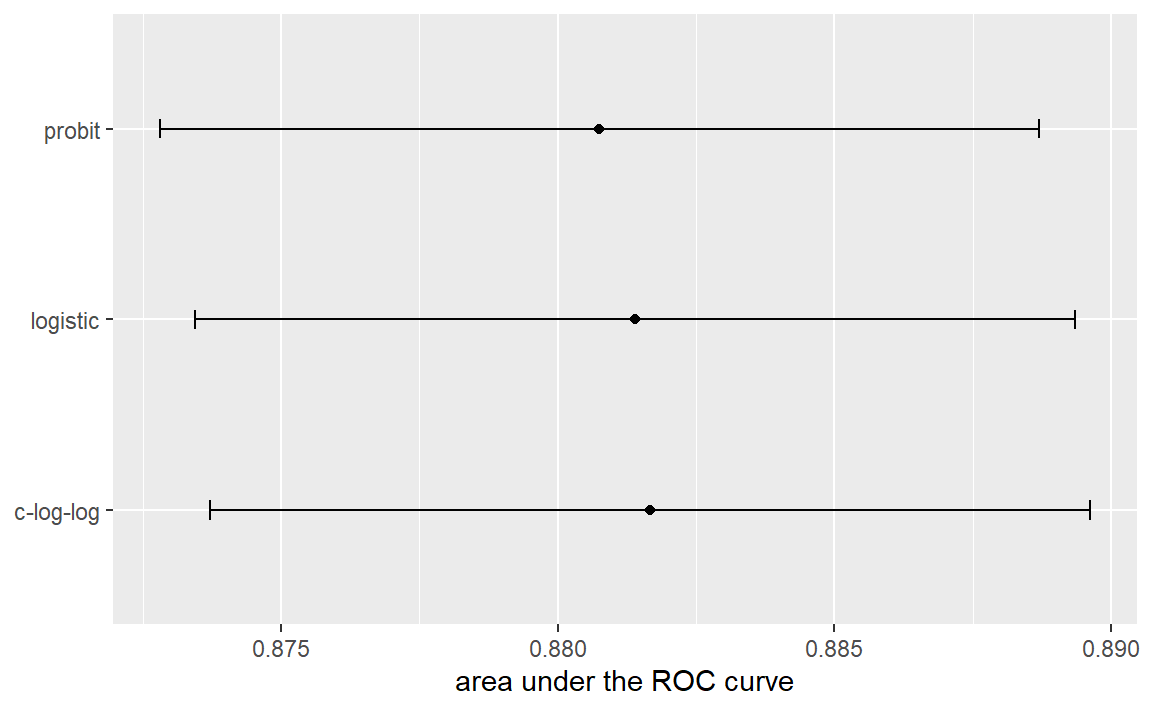
12 Model Tuning and the Dangers of Overfitting

Published

October 23, 2025

Modified

November 1, 2025

为了使用模型进行预测,必须先估计出该模型的参数。其中一些参数可以直接从训练数据中估算出来,而另一些被称为调优参数(tuning parameters)或超参数(hyperparameters)的参数,则无法直接从训练数据中获得,需事先指定。这些未知的结构化或其他类型数值对模型有重要影响,但无法通过数据直接推算。本章将提供调优参数的示例,并展示如何利用tidymodels系函数来创建和处理调优参数。此外,我们还将说明错误地选择这些值会导致过拟合(overfitting)现象,并介绍几种寻找最优调优参数值的策略。第13章和第14章将更深入地探讨用于调优的具体优化方法。

Model Parameters

在普通的线性回归中,模型有两个参数 \(\beta_0\)\(\beta_1\) :

\[ y_i = \beta_0 + \beta_1 x_i + \epsilon_i \]

当我们有结果 \(y\) 和 预测变量 \(x\) 的数据时,我们可以估计出 \(\beta_0\)\(\beta_1\)

\[ \hat \beta_1 = \frac{\sum_i (y_i-\bar{y})(x_i-\bar{x})}{\sum_i(x_i-\bar{x})^2} \]

\[ \hat \beta_0 = \bar{y}-\hat \beta_1 \bar{x} \]

对于这个示例模型,我们可以直接从数据中估计这些值,因为它们在解析上是可处理的;但在许多情况下,模型的参数无法直接从数据中估计出来。例如,对于KNN模型,给定某个输入 \(x_0\) ,它的预测值方程为:

\[ \hat y = \frac{1}{K}\sum_{\ell = 1}^K x_\ell^* \]

其中 \(K\) 是邻居的数量,而 \(x_\ell^*\) 是训练集中与 \(x_0\) 最接近的 \(K\) 个值。KNN模型由预测方程来定义,而不是模型方程。这一特性,再加上距离度量可能难以处理,使得无法创建一组可求解 \(K\) 的方程(无论是迭代求解还是通过其他方式)。邻居的数量对模型有着深远的影响,它决定了类别边界的灵活性。当 \(K\) 值较小时,边界会非常复杂;而当 \(K\) 值较大时,边界可能会相当平滑。

最近邻的数量 \(K\) 是一个很好的调优参数或超参数的例子,它无法直接从数据中估计出来。

Tuning Parameters for Different Types of Models

在不同的统计模型和机器学习模型中,存在许多调优参数或超参数的例子:

  • boosting是一种集成方法,它结合了一系列基础模型,每个基础模型都是依次创建的,并且依赖于之前的模型。boosting迭代次数是一个重要的调优参数,通常需要进行优化。

  • 在经典的单层人工神经网络(又名多层感知器)中,预测变量通过两个或多个隐藏单元进行组合。隐藏单元是预测变量的线性组合,这些组合被包含在一个激活函数(通常是一种非线性函数,如“sigmoid”函数)中。然后,隐藏单元与输出单元相连;回归模型使用一个输出单元,而分类则需要多个输出单元。隐藏单元的数量和激活函数的类型是重要的结构调优参数。

  • 现代梯度下降方法通过找到合适的优化参数得到了改进。这类超参数的例子包括学习率、动量以及优化迭代次数/轮数(Goodfellow,Bengio 和 Courville,2016)。神经网络和一些集成模型利用梯度下降来估计模型参数。虽然与梯度下降相关的调优参数并非结构参数,但它们通常需要进行调优。

在某些情况下,预处理步骤也需要调优:

  • 在主成分分析(principal component analysis)或者其有监督的“近亲”——偏最小二乘(partial least squares)中,预测变量会被替换为新的、人工构建的特征,这些特征在共线性方面具有更优的性质。提取的成分数量是可以调整的。

  • 插补方法利用一个或多个预测变量的完整值来估计缺失的预测变量值。一种有效的插补工具是使用完整列的 \(K\)-近邻 来预测缺失值。邻居的数量可以进行调整。

一些经典的统计模型也具有结构参数:

  • 在二元回归中,通常使用“logit”链接函数(即逻辑回归)。也可以使用其他链接函数,如“probit”和“complementary log-log”(Dobson,1999)。第12.3节对该示例进行了更详细的描述。

  • 非贝叶斯纵向和重复测量模型需要明确数据的协方差或相关结构。可选的结构包括复合对称(compound symmetric)(也称为可交换)、自回归(autoregressive)、托普利茨(Toeplitz)等(Littell,Pendergast 和 Natarajan,2000)。

一个不适合调整参数的例子是贝叶斯分析所需的先验分布。先验分布概括了分析师在考虑证据或数据之前对某个量的分布的信念。例如,在11.4节中,我们使用了贝叶斯方差分析模型,并且不确定回归参数的先验分布应该是什么(除了是对称分布之外)。我们选择了自由度为1的t分布作为先验分布,因为它具有更厚的尾部;这反映了我们额外的不确定性。我们的先验信念不应受到优化的影响。调优参数通常是为了优化性能而进行调整的,而先验分布不应为了得到“正确的结果”而被修改。另一个(或许更有争议的)不需要调整参数的例子是随机森林或装袋模型(bagging model)中树的数量。这个值应该选得足够大,以确保结果的数值稳定性;并且只要该值足够大,就能够产生可靠的结果,无需调整它来提升性能。随机森林通常需要数千棵树,而装袋模型所需的数量大约在50到100棵之间。

What do we Optimize?

在优化调优参数时,我们应该如何评估模型呢?这取决于模型本身以及模型的用途。

对于调优参数的统计特性易于处理的情况,可以将常见的统计特性用作目标函数。例如,在二元逻辑回归中,可以通过最大化似然函数或信息准则来选择链接函数。然而,这些统计特性可能与使用面向准确性的特性所得到的结果不一致。例如,Friedman(2001)对提升树集成中的树的数量进行了优化,发现在最大化似然函数和最大化准确性时得到了不同的结果:通过过拟合降低似然性实际上会提高错误分类率,尽管这可能违反直觉,但并不矛盾;似然性和错误率是拟合质量在不同方面的描述。

为了说明这一点,考虑 Figure 1 中所示的分类数据,其中包含两个预测变量、两个类别,共593个数据点的训练集。

#> ── Attaching packages ─────────────────────────────────── tidymodels 1.4.1 ──
#> ✔ broom        1.0.9     ✔ recipes      1.3.1
#> ✔ dials        1.4.2     ✔ rsample      1.3.1
#> ✔ dplyr        1.1.4     ✔ tailor       0.1.0
#> ✔ ggplot2      3.5.2     ✔ tidyr        1.3.1
#> ✔ infer        1.0.9     ✔ tune         2.0.0
#> ✔ modeldata    1.5.1     ✔ workflows    1.3.0
#> ✔ parsnip      1.3.3     ✔ workflowsets 1.1.1
#> ✔ purrr        1.1.0     ✔ yardstick    1.3.2
#> ── Conflicts ────────────────────────────────────── tidymodels_conflicts() ──
#> ✖ purrr::discard() masks scales::discard()
#> ✖ dplyr::filter()  masks stats::filter()
#> ✖ dplyr::lag()     masks stats::lag()
#> ✖ recipes::step()  masks stats::step()
Figure 1: An example two-class classification data set with two predictors

我们可以先为这些数据拟合一个线性分类边界。最常用的方法是使用广义线性模型,其形式为逻辑回归。该模型通过“logit”函数将样本属于类别1的对数几率联系起来:

\[ \log\left(\frac{\pi}{1 - \pi}\right) = \beta_0 + \beta_1x_1 + \ldots + \beta_px_p \]

在广义线性模型的背景下,“logit”函数是结果(\(\pi\))和预测变量之间的连接函数。还有其他连接函数,包括“probit”函数,其中 \(\Phi\) 是累积标准正态函数,:

\[ \Phi^{-1}(\pi) = \beta_0 + \beta_1x_1 + \ldots + \beta_px_p \]

还有“complementary log-log”函数:

\[ \log(-\log(1-\pi)) = \beta_0 + \beta_1x_1 + \ldots + \beta_px_p \]

上述模型都会产生线性分类边界,我们应该使用哪一个呢?因为上述模型参数的数量是不变的,我们可以计算每个模型在统计学上的(对数)似然值,并确定具有最大似然值的模型。传统上,似然值的计算需要使用与估计参数相同的数据,而不是使用像第5章和第10章中的数据拆分或重抽样之类的方法获得的数据。

对于数据框training_set,我们来创建一个函数,用于计算不同的模型并提取训练集的似然统计量(使用broom::glance()):

llhood <- function(...) {
  logistic_reg() %>%
    set_engine("glm", ...) %>%
    fit(Class ~ ., data = training_set) %>%
    glance() %>%
    select(logLik)
}

bind_rows(
  llhood(),
  llhood(family = binomial(link = "probit")),
  llhood(family = binomial(link = "cloglog"))
) %>%
  mutate(link = c("logit", "probit", "c-log-log")) %>%
  arrange(desc(logLik))
#> # A tibble: 3 × 2
#>   logLik link     
#>    <dbl> <chr>    
#> 1  -258. logit    
#> 2  -262. probit   
#> 3  -270. c-log-log

根据这些结果,逻辑回归模型具有最佳的统计特性。但从对数似然值的量级来看,很难判断这些差异是重要的还是可以忽略的。改进这种分析的一种方法是对统计数据进行重采样,并将建模数据与用于性能评估的数据分开。对于这个小数据集,重复10折交叉验证是重采样的一个不错选择。在yardstick包中,mn_log_loss()函数用于估计负对数似然,我们的结果如 Figure 2 所示。

set.seed(1201)
rs <- vfold_cv(training_set, repeats = 10)

# Return the individual resampled performance estimates:
lloss <- function(...) {
  perf_meas <- metric_set(roc_auc, mn_log_loss)

  logistic_reg() %>%
    set_engine("glm", ...) %>%
    fit_resamples(Class ~ A + B, rs, metrics = perf_meas) %>%
    collect_metrics(summarize = FALSE) %>%
    select(id, id2, .metric, .estimate)
}

resampled_res <-
  bind_rows(
    lloss() %>% mutate(model = "logistic"),
    lloss(family = binomial(link = "probit")) %>% mutate(model = "probit"),
    lloss(family = binomial(link = "cloglog")) %>% mutate(model = "c-log-log")
  ) %>%
  # Convert log-loss to log-likelihood:
  mutate(.estimate = ifelse(.metric == "mn_log_loss", -.estimate, .estimate)) %>%
  group_by(model, .metric) %>%
  summarize(
    mean = mean(.estimate, na.rm = TRUE),
    std_err = sd(.estimate, na.rm = TRUE) / sqrt(n()),
    .groups = "drop"
  )
#> → A | warning: glm.fit: fitted probabilities numerically 0 or 1 occurred
#> There were issues with some computations   A: x1
#> 

resampled_res %>%
  filter(.metric == "mn_log_loss") %>%
  ggplot(aes(x = mean, y = model)) +
  geom_point() +
  geom_errorbar(aes(xmin = mean - 1.64 * std_err, xmax = mean + 1.64 * std_err),
    width = .1
  ) +
  labs(y = NULL, x = "log-likelihood")
Figure 2: Means and approximate 90% confidence intervals for the resampled binomial log-likelihood with three different link functions

这些值的规模与之前的值不同,因为它们是在更小的数据集上计算得出的;broom::glance()产生的值是总和,而yardstick::mn_log_loss()产生的值是平均值。

换一个不同的指标怎么样?我们还计算了每个重采样的ROC曲线下面积。这些结果反映了模型在众多概率阈值下的判别能力,在 Figure 3 中显示出没有差异。

resampled_res %>%
  filter(.metric == "roc_auc") %>%
  ggplot(aes(x = mean, y = model)) +
  geom_point() +
  geom_errorbar(aes(xmin = mean - 1.64 * std_err, xmax = mean + 1.64 * std_err),
    width = .1
  ) +
  labs(y = NULL, x = "area under the ROC curve")
Figure 3: Means and approximate 90% confidence intervals for the resampled area under the ROC curve with three different link functions
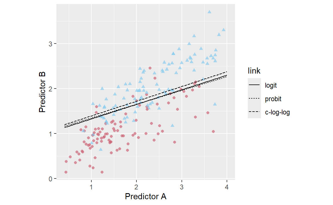
考虑到区间的重叠以及x轴的刻度,这些选项中的任何一个都可以使用。当三个模型的类别边界叠加在 Figure 4 中的198个数据点的测试集上时,我们再次看到了这一点。

data_grid <- crossing(A = seq(0.4, 4, length = 200), B = seq(.14, 3.9, length = 200))

logit_pred <-
  logistic_reg() %>%
  set_engine("glm") %>%
  fit(Class ~ A + B, data = training_set) %>%
  predict(data_grid, type = "prob") %>%
  bind_cols(data_grid) %>%
  mutate(link = "logit")

probit_pred <-
  logistic_reg() %>%
  set_engine("glm", family = binomial(link = "probit")) %>%
  fit(Class ~ A + B, data = training_set) %>%
  predict(data_grid, type = "prob") %>%
  bind_cols(data_grid) %>%
  mutate(link = "probit")

cloglog_pred <-
  logistic_reg() %>%
  set_engine("glm", family = binomial(link = "cloglog")) %>%
  fit(Class ~ A + B, data = training_set) %>%
  predict(data_grid, type = "prob") %>%
  bind_cols(data_grid) %>%
  mutate(link = "c-log-log")

link_grids <-
  bind_rows(logit_pred, probit_pred, cloglog_pred) %>%
  mutate(link = factor(link, levels = c("logit", "probit", "c-log-log")))

link_grids %>%
  ggplot(aes(x = A, y = B)) +
  geom_point(
    data = testing_set, aes(color = Class, pch = Class),
    alpha = 0.7, show.legend = FALSE
  ) +
  geom_contour(aes(z = .pred_Class1, lty = link), breaks = 0.5, color = "black") +
  scale_color_manual(values = c("#CC6677", "#88CCEE")) +
  coord_equal() +
  labs(x = "Predictor A", y = "Predictor B")
Figure 4: The linear class boundary fits for three link functions
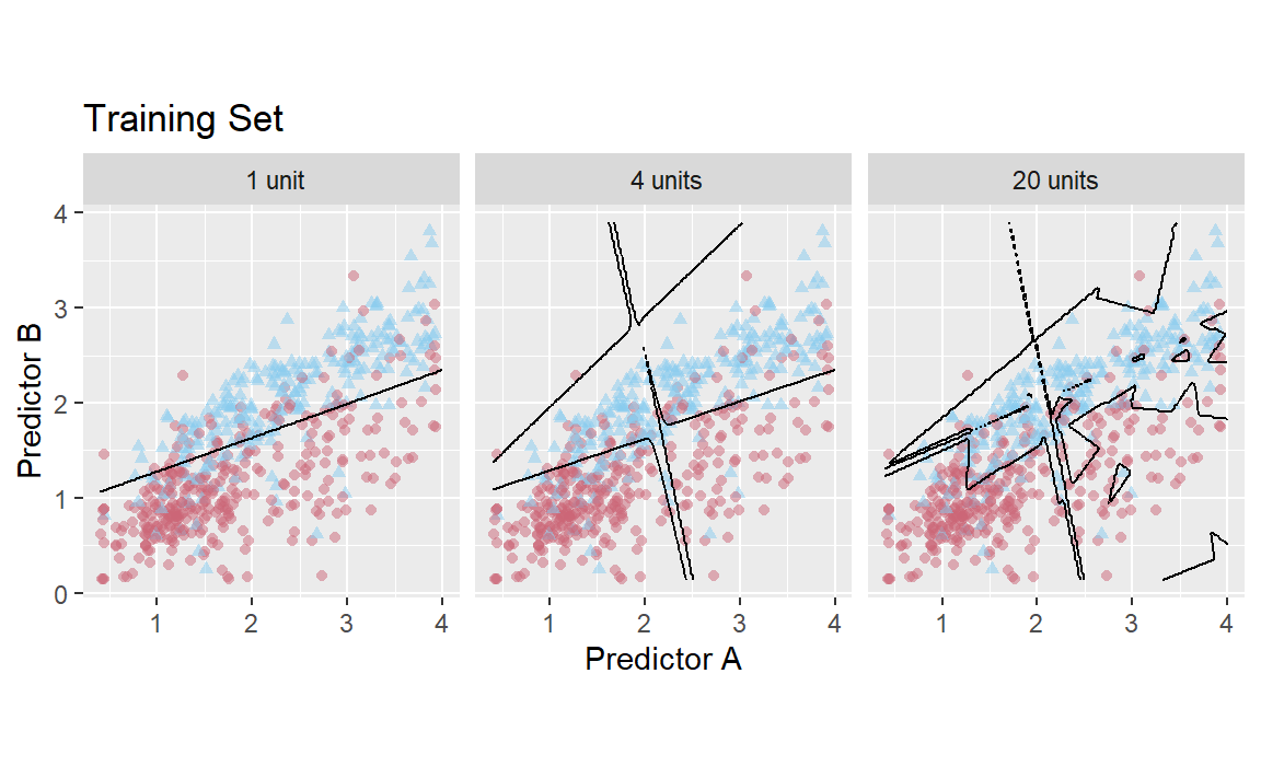
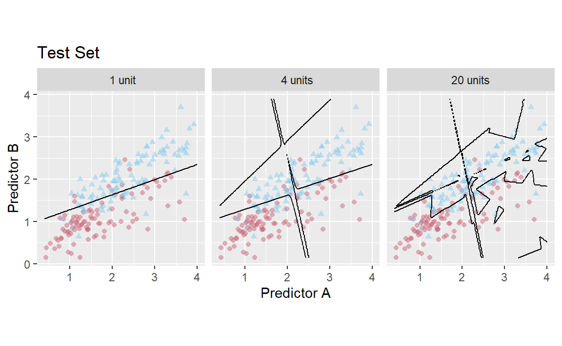
本练习强调,不同的指标可能会导致在选择调优参数值时做出不同的决策。在这种情况下,一个指标表明这些模型存在一定差异,而另一个指标则显示它们完全没有差异。Thomas 和 Uminsky(2020)对指标优化进行了深入探讨,他们研究了几个问题,包括指标的博弈。他们警告说:当前人工智能方法中,指标优化的不合理有效性是该领域面临的一项根本性挑战,并且由此产生了一个内在矛盾:仅仅优化指标会导致结果远非最优。

The consequences of poor parameter estimates

许多调优参数会调节模型复杂度的大小,更高的复杂度通常意味着模型在模拟模式时具有更强的可塑性(malleability)。例如,如第8.4.3节所示,在样条函数中增加自由度会提高预测方程的复杂性。虽然当数据中有潜在的复杂模式时,这是一个优势,但它也可能导致对偶然模式的过度解读,而这些偶然模式在新数据中不会重现。过拟合指的是模型过度适应训练数据的情况:它在用于构建模型的数据上表现良好,但在新数据上表现不佳。由于调优模型参数会增加模型的复杂度,不当的选择可能会导致过拟合。

回顾12.2节中描述的单层神经网络模型。对于分类任务的神经网络,当它只有一个隐藏单元且采用“sigmoidal”激活函数时,实际上就等同于逻辑回归。然而,随着隐藏单元数量的增加,模型的复杂度也会随之提高。事实上,当网络模型使用“sigmoidal”激活单元时,Cybenko(1989)证明,只要有足够多的隐藏单元,该模型就是一个通用函数逼近器。

我们将神经网络分类模型应用于上一节中的数据,并改变隐藏单元的数量。以ROC曲线下面积作为性能指标,随着添加的隐藏单元数量增多,模型在训练集上的效果会提升。该网络模型会彻底且细致地学习训练集。如果模型根据训练集的ROC值来评判自身,它会倾向于选择大量隐藏单元,以便几乎消除误差。

第5章和第10章表明,仅对训练集进行重新预测是一种糟糕的模型评估方法。在这里,神经网络会很快开始过度解读它在训练集中看到的模式。请比较 Figure 5 中这三个示例分类边界(基于训练集开发)在训练集和测试集上的叠加情况。

two_class_rec <-
  recipe(Class ~ ., data = two_class_dat) %>%
  step_normalize(all_numeric_predictors())

mlp_mod <-
  mlp(hidden_units = tune(), epochs = 1000) %>%
  set_engine("nnet") %>%
  set_mode("classification")

mlp_wflow <-
  workflow() %>%
  add_recipe(two_class_rec) %>%
  add_model(mlp_mod)

mlp_res <-
  tibble(
    hidden_units = 1:20,
    train = NA_real_,
    test = NA_real_,
    model = vector(mode = "list", length = 20)
  )

for (i in 1:nrow(mlp_res)) {
  set.seed(27)
  tmp_mod <-
    mlp_wflow %>%
    finalize_workflow(mlp_res %>% slice(i) %>% select(hidden_units)) %>%
    fit(training_set)
  mlp_res$train[i] <-
    roc_auc_vec(training_set$Class, predict(tmp_mod, training_set, type = "prob")$.pred_Class1)
  mlp_res$test[i] <-
    roc_auc_vec(testing_set$Class, predict(tmp_mod, testing_set, type = "prob")$.pred_Class1)
  mlp_res$model[[i]] <- tmp_mod
}

te_plot <-
  mlp_res %>%
  slice(c(1, 4, 20)) %>%
  mutate(
    probs = map(model, ~ bind_cols(data_grid, predict(.x, data_grid, type = "prob")))
  ) %>%
  dplyr::select(hidden_units, probs) %>%
  unnest(cols = c(probs)) %>%
  mutate(
    label = paste(format(hidden_units), "units"),
    label = ifelse(label == " 1 units", " 1 unit", label)
  ) %>%
  ggplot(aes(x = A, y = B)) +
  geom_point(
    data = testing_set, aes(color = Class, pch = Class),
    alpha = 0.5, show.legend = FALSE
  ) +
  geom_contour(aes(z = .pred_Class1), breaks = 0.5, color = "black") +
  scale_color_manual(values = c("#CC6677", "#88CCEE")) +
  facet_wrap(~label, nrow = 1) +
  coord_equal() +
  ggtitle("Test Set") +
  labs(x = "Predictor A", y = "Predictor B")

tr_plot <-
  mlp_res %>%
  slice(c(1, 4, 20)) %>%
  mutate(
    probs = map(model, ~ bind_cols(data_grid, predict(.x, data_grid, type = "prob")))
  ) %>%
  dplyr::select(hidden_units, probs) %>%
  unnest(cols = c(probs)) %>%
  mutate(
    label = paste(format(hidden_units), "units"),
    label = ifelse(label == " 1 units", " 1 unit", label)
  ) %>%
  ggplot(aes(x = A, y = B)) +
  geom_point(
    data = training_set, aes(color = Class, pch = Class),
    alpha = 0.5, show.legend = FALSE
  ) +
  geom_contour(aes(z = .pred_Class1), breaks = 0.5, color = "black") +
  scale_color_manual(values = c("#CC6677", "#88CCEE")) +
  facet_wrap(~label, nrow = 1) +
  coord_equal() +
  ggtitle("Training Set") +
  labs(x = "Predictor A", y = "Predictor B")

tr_plot
te_plot
(a) Training set
(b) Test set
Figure 5: Class boundaries for three models with increasing numbers of hidden units. The boundaries are fit on the training set and shown for the training and test sets.

一个隐藏单元的模型因为受限于线性,不能灵活地适应数据。具有四个隐藏单元的模型开始出现过拟合迹象,对于偏离数据主流的值,其边界不切实际。这是由数据右上角第一类中的单个数据点引起的。到20个隐藏单元时,模型开始记住训练集,在这些数据周围创建小的“孤岛”,以最小化重代入错误率。这些模式在测试集中不会重现。最后一个面板最能说明,必须控制调节复杂度的调优参数,才能使模型有效。对于20单元模型,训练集的AUC为0.944,但测试集的值为0.855。

当我们有两个可以绘图的预测变量时,这种过拟合现象是很明显的。然而,一般来说,我们必须使用定量方法来检测过拟合。可以使用样本外数据来检测模型是否在训练集上过拟合。同样,我们不能使用测试集,而是需要某种形式的重采样,这可能意味着一种迭代方法(例如,10折交叉验证)或单一数据源(例如,验证集)。

Two general strategies for optimization

调优参数优化通常分为两类:网格搜索(grid search)和迭代搜索(iterative search)。

网格搜索是指我们预先定义一组要评估的参数值。网格搜索涉及的主要选择是如何构建网格以及要评估多少种参数组合。网格搜索通常被认为效率低下,因为随着“维度灾难”的出现,覆盖参数空间所需的网格点数量可能会变得难以处理。这种担忧有一定道理,在流程未优化时尤为明显。第13章对此有更详细的讨论。

迭代搜索或顺序搜索是指我们基于先前的结果依次发现新的参数组合。几乎任何非线性优化方法都是适用的,在某些情况下,需要一组初始的一个或多个参数组合的结果来启动优化过程。第14章将对迭代搜索进行更详细的讨论。

Figure 6 展示了两个面板,这两个面板针对具有两个在0到1之间取值的调优参数的情况,演示了这两种方法。在每个面板中,一组等高线显示了参数与结果之间真实的(模拟的)关系。最优结果位于右上角。

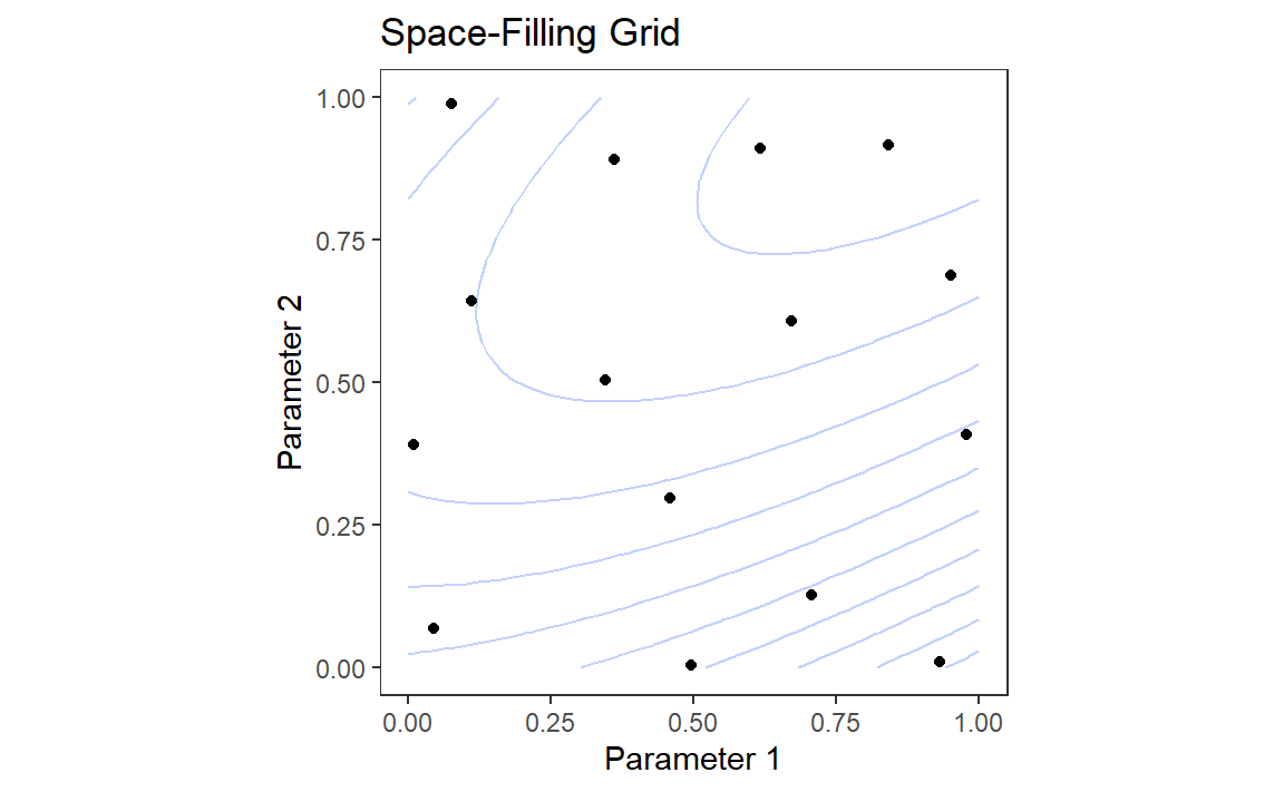
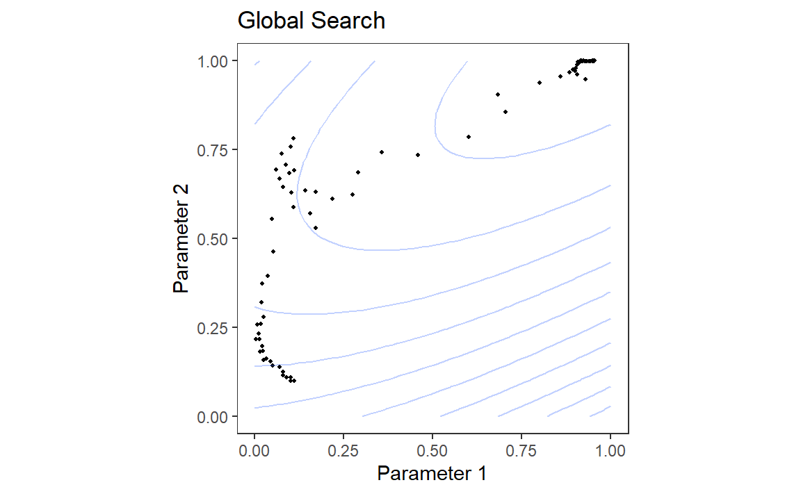
# load("E:/Blog/Books/Tidy Modeling with R/Rdata/search_examples.RData")
load("./Rdata/search_examples.RData")

grid_plot <-
  ggplot(sfd_grid, aes(x = x, y = y)) +
  geom_point() +
  lims(x = 0:1, y = 0:1) +
  labs(x = "Parameter 1", y = "Parameter 2", title = "Space-Filling Grid") +
  geom_contour(
    data = grid_contours,
    aes(z = obj),
    alpha = .3,
    bins = 12
  ) +
  coord_equal() +
  theme_bw() +
  theme(
    panel.grid.major = element_blank(),
    panel.grid.minor = element_blank()
  )

search_plot <-
  ggplot(nm_res, aes(x = x, y = y)) +
  geom_point(size = .7) +
  lims(x = 0:1, y = 0:1) +
  labs(x = "Parameter 1", y = "Parameter 2", title = "Global Search") +
  coord_equal() +
  geom_contour(
    data = grid_contours,
    aes(x = x, y = y, z = obj),
    alpha = .3,
    bins = 12
  ) +
  theme_bw() +
  theme(
    panel.grid.major = element_blank(),
    panel.grid.minor = element_blank()
  )

grid_plot
search_plot
(a) Space-Filling Grid
(b) Global Search
Figure 6: Examples of pre-defined grid tuning and an iterative search method. The lines represent contours of a performance metric; it is best in the upper-right-hand side of the plot.

Figure 6 的左面板展示了一种名为空间填充设计(space-filling design)的网格类型。这是一种为覆盖参数空间的设计,其目的是使调优参数组合彼此之间不会过于接近。这种设计的结果中,没有任何点恰好位于真正的最优位置。不过,有一个点处于大致的附近区域,其性能指标结果很可能在最优值的误差范围内。

Figure 6 的右侧面板展示了一种全局搜索方法(global search method)的结果——Nelder-Mead单纯形法(奥尔森和纳尔逊,1975)。起始点位于参数空间的左下部分。搜索在空间中蜿蜒前行,直到到达最优位置,在那里它会努力尽可能接近数值上的最佳值。这种特定的搜索方法虽然有效,但并不以效率著称;它需要进行大量的函数评估,尤其是在接近最优值的地方。第14章将讨论更高效的搜索算法。

混合策略也是一种选择,并且效果很好。在初始网格搜索之后,序贯优化可以从最佳网格组合开始。这些策略的示例将在接下来的两章中详细讨论。在继续之前,让我们学习如何使用dials包在tidymodels中处理调优参数对象。

Tuning Parameters in tidymodels

在前面的章节中,我们已经讨论了相当多与recipe对象和模型的调优参数相对应的参数。以下这些参数是可以进行调优的:

  • 将社区合并为“其他”类别的阈值(参数名称为threshold),在第8.4.1节中进行了讨论

  • 自然样条中的自由度数量(deg_free,第8.4.3节)

  • 在基于树的模型中执行分割所需的数据点数量(min_n,第6.1节)

  • 惩罚模型中的正则化量(penalty,第6.1节)

由parsnip包构建的模型函数,有两种参数:

  • 主要参数(main arguments):为了性能而进行优化且在多个引擎中可用的常见参数,它们是模型函数的顶级参数,例如,rand_forest()函数有主要参数treesmin_nmtry,因为这些参数是最常被指定或优化的。

  • 特定于引擎(调优参数)的调优参数:这些参数要么很少被优化,要么只针对某些特定引擎。例如,随机森林ranger包有一些其他包不会使用的参数,比如“增益惩罚”——它在树的归纳过程中对预测因子的选择进行正则化,这个参数有助于调节集成中使用的预测因子数量与性能之间的权衡(Wundervald、Parnell和Domijan,2020)。在ranger()中,这个参数的名称是regularization.factor。要通过parsnip模型规格指定一个值,需将其作为补充参数添加到set_engine()中:

rand_forest(trees = 2000, min_n = 10) %>%                   # <- main arguments
  set_engine("ranger", regularization.factor = 0.5)         # <- engine-specific

主要参数使用统一的命名系统,以消除不同引擎之间的不一致性,而特定于引擎的参数则不这样做。

我们如何向tidymodels函数表明哪些参数需要优化?通过为参数赋值tune()来标记需要调整的参数。对于第12.4节中使用的单层神经网络,隐藏单元的数量通过以下方式指定为需要调整的参数:

neural_net_spec <-
  mlp(hidden_units = tune()) %>%
  set_mode("regression") %>%
  set_engine("keras")

tune()函数不会执行任何特定的参数值;它只返回一个表达式:

tune()
#> tune()

将这个tune()值嵌入到参数中,会为待优化的参数添加标签。接下来两章中展示的模型调优函数会解析模型和recipe对象,以发现带有标签的参数。这些函数能够自动配置和处理这些参数,因为它们了解这些参数的特性(例如,值的范围等)。

extract_parameter_set_dials(neural_net_spec)
#> Collection of 1 parameters for tuning
#> 
#>    identifier         type    object
#>  hidden_units hidden_units nparam[+]
#> 

结果显示值为nparam[+],这表明隐藏单元的数量是一个数值参数。

有一个可选的标识参数,用于将名称与参数相关联。当同一种参数在不同地方进行调优时,这会很有用。例如,对于10.6节中的Ames房产数据,recipe对象使用样条函数对经度和纬度都进行了编码。如果我们想调优这两个样条函数,使其可能具有不同的平滑度,我们会调用两次step_ns(),每个预测变量调用一次。为了使这些参数可识别,标识参数可以采用任何字符串:

data(ames)
ames <- mutate(ames, Sale_Price = log10(Sale_Price))
set.seed(502)
ames_split <- initial_split(ames, prop = 0.80, strata = Sale_Price)
ames_train <- training(ames_split)
ames_test <- testing(ames_split)

ames_rec <-
  recipe(Sale_Price ~ Neighborhood + Gr_Liv_Area + Year_Built + Bldg_Type +
    Latitude + Longitude, data = ames_train) %>%
  step_log(Gr_Liv_Area, base = 10) %>%
  step_other(Neighborhood, threshold = tune()) %>%
  step_dummy(all_nominal_predictors()) %>%
  step_interact(~ Gr_Liv_Area:starts_with("Bldg_Type_")) %>%
  step_ns(Longitude, deg_free = tune("longitude df")) %>%
  step_ns(Latitude, deg_free = tune("latitude df"))

recipes_param <- extract_parameter_set_dials(ames_rec)
recipes_param
#> Collection of 3 parameters for tuning
#> 
#>    identifier      type    object
#>     threshold threshold nparam[+]
#>  longitude df  deg_free nparam[+]
#>   latitude df  deg_free nparam[+]
#> 

请注意,identifier列和type列对于这两个样条参数来说并不相同。

当使用工作流将recipe对象和模型结合起来时,两组参数都会显示:

wflow_param <-
  workflow() %>%
  add_recipe(ames_rec) %>%
  add_model(neural_net_spec) %>%
  extract_parameter_set_dials()
wflow_param
#> Collection of 4 parameters for tuning
#> 
#>    identifier         type    object
#>  hidden_units hidden_units nparam[+]
#>     threshold    threshold nparam[+]
#>  longitude df     deg_free nparam[+]
#>   latitude df     deg_free nparam[+]
#> 

神经网络极其擅长模拟非线性模式。向这类模型中添加样条项是没有必要的;我们将此模型与recipe对象结合起来只是为了举例说明。

每个调优参数在dials包中都有一个对应的函数。在绝大多数情况下,该函数与参数参数同名:

hidden_units()
#> # Hidden Units (quantitative)
#> Range: [1, 10]
threshold()
#> Threshold (quantitative)
#> Range: [0, 1]

deg_free参数是一个反例;自由度的概念会出现在各种各样不同的语境中。当用于样条函数时,有一个专门的dials函数叫做spline_degree(),默认情况下,它会被用于样条函数:

spline_degree()
#> Spline Degrees of Freedom (quantitative)
#> Range: [1, 10]

dials包还提供了一个便捷函数,用于提取特定的参数对象:

# identify the parameter using the id value:
wflow_param %>% extract_parameter_dials("threshold")
#> Threshold (quantitative)
#> Range: [0, 0.1]

在参数集中,参数的范围也可以就地更新:

extract_parameter_set_dials(ames_rec) %>%
  update(threshold = threshold(c(0.8, 1.0)))
#> Collection of 3 parameters for tuning
#> 
#>    identifier      type    object
#>     threshold threshold nparam[+]
#>  longitude df  deg_free nparam[+]
#>   latitude df  deg_free nparam[+]
#> 

extract_parameter_set_dials()创建的参数集会被tidymodels调优函数使用(在需要时)。如果需要修改调优参数对象的默认值,则将修改后的参数集传递给相应的调优函数。

一些调优参数取决于数据的维度。例如,最近邻的数量必须在1和数据的行数之间。在某些情况下,很容易为可能的取值范围设定合理的默认值。而在其他情况下,参数范围至关重要,不能随意假设。随机森林模型的主要调优参数是每个树节点分裂时随机抽样的预测变量列的数量,通常记为mtry()。在不知道预测变量数量的情况下,该参数范围无法预先配置,需要进行最终确定。

rf_spec <-
  rand_forest(mtry = tune()) %>%
  set_engine("ranger", regularization.factor = tune("regularization")) %>%
  set_mode("regression")

rf_param <- extract_parameter_set_dials(rf_spec)
rf_param
#> Collection of 2 parameters for tuning
#> 
#>      identifier                  type    object
#>            mtry                  mtry nparam[?]
#>  regularization regularization.factor nparam[+]
#> 
#> Model parameters needing finalization:
#> # Randomly Selected Predictors ('mtry')
#> 
#> See `?dials::finalize()` or `?dials::update.parameters()` for more
#> information.

完整的参数对象在其摘要中带有[+][?]值表示可能范围中至少有一端缺失。有两种处理方法。第一种是使用update(),根据你对数据维度的了解添加范围:

rf_param %>%
  update(mtry = mtry(c(1, 70)))
#> Collection of 2 parameters for tuning
#> 
#>      identifier                  type    object
#>            mtry                  mtry nparam[+]
#>  regularization regularization.factor nparam[+]
#> 

然而,如果一个recipe对象附加到使用了添加或删除列的步骤的工作流中,这种方法可能就不奏效了。如果这些步骤不计划进行调整,那么finalize()函数可以执行一次该recipe对象以获取维度:

pca_rec <-
  recipe(Sale_Price ~ ., data = ames_train) %>%
  # Select the square-footage predictors and extract their PCA components:
  step_normalize(contains("SF")) %>%
  # Select the number of components needed to capture 95% of
  # the variance in the predictors.
  step_pca(contains("SF"), threshold = .95)

updated_param <-
  workflow() %>%
  add_model(rf_spec) %>%
  add_recipe(pca_rec) %>%
  extract_parameter_set_dials() %>%
  finalize(ames_train)
updated_param
#> Collection of 2 parameters for tuning
#> 
#>      identifier                  type    object
#>            mtry                  mtry nparam[+]
#>  regularization regularization.factor nparam[+]
#> 
updated_param %>% extract_parameter_dials("mtry")
#> # Randomly Selected Predictors (quantitative)
#> Range: [1, 74]

当recipe对象准备好后,finalize()函数会学习将mtry的上限设置为74个预测变量。

此外,extract_parameter_set_dials()的结果将包含特定于引擎的参数(如果有的话)。这些参数的发现方式与主要参数相同,并被包含在参数集中。dials包包含所有可能可调节的特定于引擎的参数的参数函数:

rf_param
#> Collection of 2 parameters for tuning
#> 
#>      identifier                  type    object
#>            mtry                  mtry nparam[?]
#>  regularization regularization.factor nparam[+]
#> 
#> Model parameters needing finalization:
#> # Randomly Selected Predictors ('mtry')
#> 
#> See `?dials::finalize()` or `?dials::update.parameters()` for more
#> information.
regularization_factor()
#> Gain Penalization (quantitative)
#> Range: (0, 1]

最后,有些调优参数最好与转换相关联。一个很好的例子是与许多正则化回归模型相关的惩罚参数。该参数是非负的,通常以对数单位改变其值。主要的dials参数对象表明默认使用转换:

penalty()
#> Amount of Regularization (quantitative)
#> Transformer: log-10 [1e-100, Inf]
#> Range (transformed scale): [-10, 0]

了解这一点很重要,尤其是在更改范围时。新的范围值必须采用转换后的单位:

# correct method to have penalty values between 0.1 and 1.0
penalty(c(-1, 0)) %>%
  value_sample(1000) %>%
  summary()
#>    Min. 1st Qu.  Median    Mean 3rd Qu.    Max. 
#>  0.1002  0.1796  0.3284  0.4007  0.5914  0.9957

# incorrect:
penalty(c(0.1, 1.0)) %>%
  value_sample(1000) %>%
  summary()
#>    Min. 1st Qu.  Median    Mean 3rd Qu.    Max. 
#>   1.261   2.081   3.437   4.151   5.781   9.996

如果需要,可以通过trans参数更改尺度。你可以使用自然单位,但要保持相同的范围:

penalty(trans = NULL, range = 10^c(-10, 0))
#> Amount of Regularization (quantitative)
#> Range: [1e-10, 1]

Chapter Summary

本章介绍了模型超参数的调优过程,这些超参数无法直接从数据中估计出来。调整这类参数可能会导致过拟合,这通常是因为模型变得过于复杂,所以使用重采样数据集以及适当的评估指标非常重要。确定合适值有两种通用策略,即网格搜索和迭代搜索,我们将在接下来的两章中深入探讨。在tidymodels中,tune()函数用于确定待优化的参数,而dials包中的函数可以提取调优参数对象并与之交互。

Back to top